So, I am reading this book called “Probability Theory; The logic of Science” by E.T. Jaynes. It is an excellent read, highly recommended, and quite an eye-opener to me in terms of understanding statistics and data analysis from first principles. Here I am sharing a few particularly interesting insights from chapter 9.11 (“Significance Tests”, p. 293).

A simple experiment

A p-value gives, in deliberately vague terms, the degree to which some ‘Null-Hypothesis’ is consistent with the data. For example, let’s say we perform an experiment of 100 repeated coin tosses, yielding 55 heads and 45 tails. As ‘Null-hypothesis’, we denote the hypothesis that the coin was ‘fair’ and that the experiment was performed in a fair manner, with the same expected frequency of 50% for both heads and tails (As a side remark, note that ‘fair’ in these assumptions is actually very difficult to define without circularity, which is another topic covered in the book). We can then compute a p-value for the Null-hypothesis given the observed data, which in this case turns out to be (Binomial tail-test)

$$p=2 \sum_{k=55}^{100}\binom{100}{k}\left(\frac{1}{2}\right)^k \left(\frac{1}{2}\right)^{100-k}\approx 0.37$$

So given the usual significance threshold of 0.05, we would not reject the Null hypothesis and conclude that the results of the experiment are consistent with a fair coin and fair tossing.

OK, so far so good.

From a Bayesian perspective, there is a problem here. As a Bayesian, we would like to compute the posterior probability for the Null-hypothesis being true, but that is not possible if the Null-hypothesis is the only hypothesis considered. The result would always be 100%. So in Bayesian hypothesis testing, we need to talk about alternative hypotheses.

Let us try the Bayesian approach. We are going to compare the Null-hypothesis with a yet to be defined alternative hypothesis. Let us denote the Null hypothesis by H₀ and the alternative hypothesis by H₁. Giving both of them prior probability 1/2, Bayes’ theorem for H₀ then reads

$$P(H_0|D)=\frac{P(D|H_0)}{P(D|H_0)+P(D|H_1)}$$

(where D denotes the data, and P(D|H) denotes the sampling probability under hypothesis H). Now, we know what P(D|H₀) should be, it should be the binomial sampling probability as already used above. Specifically, for 55 heads out of 100 trials, and a heads-probabality of 50% under H₀, we get

$$P(D|H_0)=\binom{100}{55}\left(\frac{1}{2}\right)^{55} \left(\frac{1}{2}\right)^{100-55}\approx 0.048$$

So, what type of alternative hypothesis should we consider? If you are tempted to say “all possible alternatives”, you run into problems. For example, it is always possible to cook up some pathological hypothesis that Jaynes calls “the sure-thing hypothesis”, which has the property that P(D|H₁)=1. This hypothesis states that the observed data is exactly produced with likelihood 1, and there could not have been any other result. Such a hypothesis means that not only the correct frequencies, but also the correct order of coin tosses is predicted. Clearly, we do not want to consider this hypothesis, or rather, we would set the prior probability for such a “sure-thing hypothesis” to zero.

Instead, we would like to compare our Null-hypothesis with some set of reasonable alternative hypotheses. Specifically, the hypotheses that we would like to consider are all from the “Bernoulli-class”, which are parameterized by a real number 𝜆. These hypotheses state that i) all trials are independent, ii) at each trial, the probability for heads is 𝜆. You can see that the likelihood of the data under any such hypothesis is again binomial.

For now, to keep things more comparable to the orthodox significance test, we would like to still make pairwise comparisons and avoid considering all alternative hypotheses at the same time (which amounts to parameter estimation, see below). It would therefore be instructive to consider the best possible Bernoulli-class hypothesis as our hypothesis H₁. It is easy to show, and intuitively clear, that the best possible Bernoulli-class hypothesis for our data is the one where 𝜆 equals the observed frequency of heads in the sample. Therefore, we consider 𝜆=0.55, which leads to a binomial sampling probability of P(D|H₁)≈0.08. This then gives us a posterior probability for hypothesis H₀ of

$$P(H_0|D)=\frac{P(D|H_0)}{P(D|H_0)+P(D|H_1)}= \frac{0.048}{0.08+0.048}\approx 0.38,$$

which is very close to the p-value obtained using the Binomial tail-test (≈0.37).

For the record, this type of ‘Bayesian significance test’ is called ‘Psi-test’ in Jaynes’ book, although with a slightly different formalism. Nevertheless, I will adopt this name for this type of hypothesis test, which uses a single Null-hypothesis and compares it to the best possible Bernoulli class alternative.

So to conclude up to this point: In this simple setting, the p-value obtained from an orthodox significance test is similar to the posterior probability for the Null hypothesis compared to an implied best alternative hypothesis, which is simply the hypothesis that success probabilities equal observed success-frequencies. While our Bayesian approach can let us feel a bit smug that we have a crystal-clear interpretation of our result (as a posterior probability), there is not much of a practical difference between the two approaches in this particular case.

A more complicated experiment

Let’s now turn to the actual example in Jaynes’ book. We again consider a coin tossing experiment, but this time, there is a third possible result beyond heads (i=1) and tails (i=2): The coin can also stand on its side (i=3). Let’s say the experiment has been performed, and the results are: n₁=14, n₂=14, n₃=1. So the ‘miracle’ outcome of the coin standing on its side has been observed once.

Now, let us consider a researcher, Ms A, who knows how the coin looks and how it is tossed, and so she assigns the following probabilities for the three possible outcomes (hypothesis HA): p₁=p₂=0.499, p₃=0.002. A second person, Mr B, lives on planet Mars and has never seen a coin and has no clue how the experiment might look. However, he learns that apparently it is a repetitive experiment with three possible outcomes, so as ignorant as he is, he assigns uniform sampling probabilities to the three outcomes (hypothesis HB): (p₁=p₂=p₃=1/3).

We will now use the same approach as above, the Psi-test, and compute the posterior probabilities for both of these hypotheses, comparing them to the best Bernoulli-class alternative (still denoted H₁). First, here are the relevant sampling probabilities (likelihoods), which are now of multinomial form:

$$\begin{align} P(D|H_A)&=\frac{29!}{14!14!1!}0.499^{28}\times 0.002\approx 0.0082\\ P(D|H_B)&=\frac{29!}{14!14!1!}\left(\frac{1}{3}\right)^{29}\approx 0.000017\\ P(D|H_1)&=\frac{29!}{14!14!1!}\left(\frac{14}{29}\right)^{28} \times\frac{1}{29}\approx 0.027 \end{align} $$

So now, Ms A and Mr B both perform the Psi-test and evaluate the posterior probabilities for their respective hypotheses, compared with the best alternative hypothesis H₁. Here is what they get:

$$\begin{align} P(H_A|D)&=\frac{P(D|H_A)}{P(D|H_A)+P(D|H_1)}=\frac{0.0082}{0.0082+0.027}\approx 0.23\\ P(H_B|D)&=\frac{P(D|H_B)}{P(D|H_B)+P(D|H_1)}=\frac{0.000017}{0.000017+0.027}\approx 0.00063 \end{align}$$

So at this point, using the usual threshold of 5% for significance, Ms A concludes that the data is indeed consistent with her hypothesis. Mr B learns that his hypothesis is strongly rejected by the data, consistent with our intuition.

Psi vs. Chi-squared

Now, how does orthodox statistics deal with this scenario? Well, we have three possibilities for each trial, so we cannot anymore use the Binomial tail-test as in the simple case above. A standard tool of choice in this case is the Chi-squared statistic. It can be used for other purposes as well, but here we simply use it as a goodness-of-fit statistic. We’d like to ask how well Ms A’s and Mr B’s hypotheses are fitting the data. This Chi-squared statistic is defined as

$$\chi^2=\sum_k \frac{(n_k-np_k)^2}{p_k}$$

where nk is the number of observations with outcome k, n=∑ nk is the number of trials, and pk is the predicted frequency of the k’th 𝜒outcome. Let us compute this statistic for Ms A’s and Mr B’s hypotheses:

$$\begin{align} \chi_A^2&=2\left(\frac{(14-29\times0.499)^2}{29\times0.499}\right) +\frac{(1-29\times 0.002)^2}{29\times0.002}=15.33\\ \chi_B^2&=2\left(\frac{(14-29\times0.333)^2}{29\times0.333}\right) +\frac{(1-29\times 0.333)^2}{29\times0.333}=11.66 \end{align}$$

Amazingly, in this example Mr B obtains a lower 𝜒² value, suggesting that Mr B’s hypothesis is a better fit to the data. This clearly contradicts intuition. How is that possible? The reason is the denominator in the Chi-squared statistic, which makes it concentrate enormously on the very unlikely events. In this case, according to Ms A’s hypothesis, the most unlikely event was that the coin would be standing on it’s side (expected frequency 0.002). The fact that it was observed once in 29 tosses was a lot higher than the expectation and caused Ms A’s 𝜒² statistic to be completely inflated. Note, however, that the chance that we see an event of expected frequency 0.002 once in 29 tosses is actually not that low. Precisely, it should occur once in 29 tosses with probability 1/17.33, which is certainly a bit unlikely, but not overwhelmingly unlikely (according to the hypothesis).

We can use these values to perform an actual Chi-squared test. A p-value for this test can be computed from the 𝜒²-distribution, here with two degrees of freedom (we have three possible outcomes). We find:

$$\begin{align}p_A&=0.00047\\ p_B&=0.0029\end{align}$$

So here, Ms A would strongly reject her hypothesis, and Mr B would also reject his hypothesis, although he would find that his hypothesis is still better supported than Ms A’s. Again, this completely contradicts both intuition and the Bayesian approach, which is arguably less heuristic and more straight forward in this case.

You may object now that this is a constructed extreme example, and I would agree. But the illuminating point for me, when I read about this example, was that if a method is not based on robust first principles, you can never be fully sure on what you get. P-values sometimes do correspond to posterior probabiltiies, but sometimes they don’t. It seems to me the Bayesian approach, where the results are always posterior probabiltiies should be preferred over the classical Chi-squared approach in this case.

Hypothesis testing vs. parameter estimation

What I really like about the Psi-test is the fact that it can be used as a drop-in replacement for orthodox significance tests that are so common in science. They come closest to what orthodox statistics is so widely used for: computing p-values. However, one cannot really discuss the Bayesian method without mentioning that an even more idiomatic approach for these kind of problems would be parameter estimation.

Both experiments discussed above have data and a parameterized model. We just happened to single out one specific parameter value and called them ‘Null-hypothesis’. In the first experiment this specific parameter value was the 50% heads/tails probability for a fair coin. In the second experiment, the parameters were the multinomial probabilities for heads/tails and stand-on-its-side, and we singled out the values assigned by Ms A and Mr B.

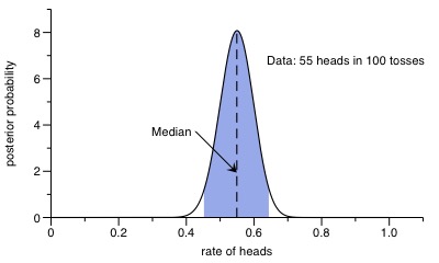
But why would we actually approach the problem with singling out specific parameter values in the first place? An even better approach would be to fully estimate the parameters from the data, open for any value including the ‘fair’ coin. This can be done using Bayes’ theorem as well. I won’t go much into detail, but simply note that the posterior distribution for a Bernoulli-process with two possible outcomes is a Beta distribution. In case of the first experiment, here is the result:

The 95% highest posterior credible interval is the region shaded in blue, and as one can see it comfortably includes the special value of 50%, representing a ‘fair’ coin. So without invoking any p-values, we could have stopped here and concluded that the experiment was consistent with a fair coin (but also with unfair coins within the shaded area).

In the second experiment, with three outcomes, the posterior distribution is a Dirichlet distribution, which is defined on a two-dimensional Simplex and more cumbersome to plot. However, the marginal distributions for the rate of heads, tails and for standing on the side are again Beta distributions that can be plotted easily. And since the data is symmetric in heads and tails (both with 14 outcomes in 29 tosses), we simply need to plot two distributions, representing heads (and tails), and for the rate of standing on its side:

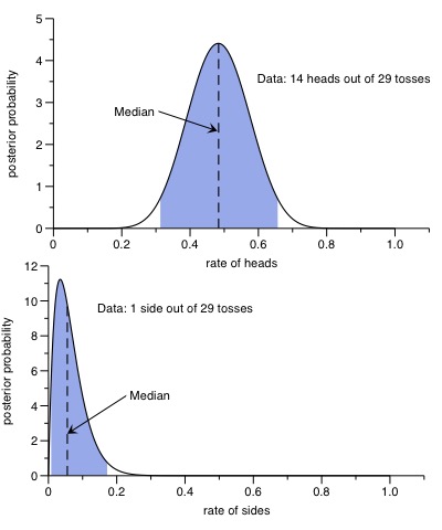
Interestingly, the posterior distribution for the rate of the coin standing on its side has its 95% highest credible interval from 0.8% up to 17%, so it excludes the rate proposed my Ms A., which was 0.2%. However, this deviation was not enough to reject the entire hypothesis with the Psi-test, since the heads- and tail-probabilities proposed by Ms A were spot on.

Conclusions

I draw three main insights from these results in Jaynes’ book:

1. There is a clean and Bayesian way to test a single Null-hypothesis without explicitly worrying about alternatives. The implicit alternative hypothesis used in this so-called Psi-test is the best possible single Bernoulli-class hypothesis. I have not seen this approach used ever in scientific papers I have read, and I wonder why. Its clean interpretation as the posterior probability for the Null-hypothesis seems very attractive to me, and preferable over any tail-test involving sampling frequencies, which seem sometimes a bit adhoc to me.
2. Chi-squared tests can sometimes give absurd results, in situations where the Bayesian approach works just fine. Perhaps experts know inuitively when and when not to use it, to avoid pitfalls such as the one presented here. But for me, being trained more in thinking in terms of probability than orthodox statistical methods, it is comforting that a Bayesian approach, for example using the Psi-test, ‘does the right thing’ always. There is no interpretation bottleneck in Bayesian probability theory, as the results are always a clean probability distribution and as such can directly be used to reflect our belief about the truth.
3. Parameter estimation is for me still the preferred way to deal with problems such as the ones presented here. As shown, plotting a posterior distribution is the most honest way to present our belief about underlying models, more so than presenting a single p-value, whether obtained via tail tests or a Psi-test. But I recognize that classical hypothesis testing of a single Null-hypothesis is so widely used in Science, that it is often easier to claim rejection or consistency of a model with a single p-value, rather than presenting credible intervals of entire distributions. For these cases, I would consider using the Psi-test in the future.